Extracting location data from the loc.gov API for geovisualization#
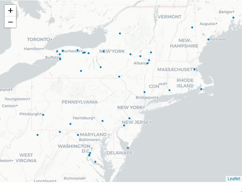
This notebook will cover how to extract location data from the loc.gov API using Python, and create a visualization as shown below. Embedded within digital collections available from the Library of Congress website are geographic data, including the locations of items and their local contexts. Digital mapping has become an increasingly accessible and valuable complement to traditional interpretive narratives. Working with spatially-referenced data offers exciting possibilities for placed-based scholarship, outreach, and teaching. It’s also a perfect avenue for interdisciplinary collaboration — between, say, humanities researchers new to GIS and spatial scientists who’ve been using it for decades. We will cover the following:
Version#
Version: 2
Last Run: July 2, 2025 (Python 3.12)
Author Information:
Written by Charlie Moffet, LC Labs Innovation Intern 2018
Edited by Sabrina Templeton, Junior Fellow 2025
Prerequisites#
In order to run this notebook, you will need to have a few Python packages installed, including the folium package which we use to create the final visualization and the pandas package for data manipulation. If any of these packages are not installed in your environment, you can install them using pip install [package-name].
Background on the data#
The story of the data we will use today would be incomplete without a critical understanding of the history behind their collection and stewardship. In this tutorial, we demonstrate how loc.gov JSON API users can find and store spatial information from Library content with an awareness toward data quality, provenance, and why this broadened scope is important for informing research projects at the Library.
Rights and access
Rights and restrictions, including copyright, affect how you can use images, particularly if you want to publish, display, or otherwise distribute them. You can read more about copyright and other restrictions that apply to the publication/distribution of images from the Prints & Photographs Division (P&P) at this link: https://guides.loc.gov/p-and-p-rights-and-restrictions/risk-assessment
The records in the case study that follows were created for the U.S. Government and are considered to be in the public domain. It is understood that access to this material rests on the condition that should any of it be used in any form or by any means, the author of such material and the Historic American Engineering Record of the Heritage Conservation and Recreation Service at all times be given proper credit.
Data quality
Consistency and accuracy of geographic information stored with digital content on the Library of Congress website varies across and within collections. This tutorial was designed as a method of exploring existing spatial references for items. Finding and analyzing meaningful patterns from secondary data typically requires additional data corrections, contexts, and geocoding frameworks to ensure optimal coverage and accuracy. The same applies to spatial data analysis involving digital collections at the Library of Congress; in any case, time spent analyzing and interpeting data is mostly spent cleaning and grappling with the data. Rather than gloss over it, here we elect to revel in that critical stage of research to both demonstrate a particular subset of techniques, and to appreciate its nuances and implications.
Further background
As a graduate student of applied urban science, I was inspired at the outset of my internship with LC Labs to discover content about the built environment across US cities on the Library website. What I found was an expansive dataset of digitized photographs, drawings and reports recognized collectively as the HHH, which includes material from three programs:
Historic American Buildings Survey (HABS)
Historic American Engineering Record (HAER)
Historic American Landscapes Survey (HALS)
More about HHH: https://www.loc.gov/collections/historic-american-buildings-landscapes-and-engineering-records/about-this-collection/
Browsing the collection:

Example of material found in the collection:
View of the uptown platform at 79th Street. Photo by David Sagarin for the Historical American Engineering Record, Library of Congress, Prints and Photographs Division, August 1978.

I decided to dig a bit deeper into the engineering record because it appeared to have the best coverage of the three for spatial references. The Historic American Engineering Record, or HAER, was established in partnership by the National Park Service (NPS), the American Society of Civil Engineers and the Library of Congress in 1969. There are more than 10,000 HAER surveys of historic sites and structures related to engineering and industry. The collection is an ongoing effort with established guidelines for documentation – HAER was created to preserve these structures through rule-based documentation, and those documents have in turn been preserved through time.
Read more about HAER Guidelines here: https://www.nps.gov/subjects/heritagedocumentation/guidelines.htm
Context#
As happens often with classifications, there are records that could rightly be placed under more than one program. There are many sites documented under the Historic American Building Surveys (HABS) that if recorded today would be assigned under HAER. Bridges are one key example. Before HAER was established, engineering-related structures, manufacturing and industrial sites, processes, watercraft, bridges, vehicles, etc. were documented under HABS. What I’ve aimed to develop here, as a result of both my own investigation as well as conversations with Library staff, is a flexible and reproducible approach to looking at the implications for scholarship of changes to preservation over time.
Geography was actually the motivating factor behind how these materials were originally organized by NPS and the Library of Congress. In the 1930s, HABS surveyors were organized into district offices that documented one or more states. The materials that they created usually (not always, which is a different problem) included state/county/city. While the Park Service played a leading role in documenting geographic data, the Library of Congress also shaped the material in the process of archiving the surveys.
The Library of Congress uses two systems to organize HABS/HAER/HALS documentation: The newer system uses the survey number as the call number. The older system assigned each survey a call number based on its location (state/county/city). Ex: HABS AL-654 has the call number: HABS ALA,1-PRAVI.V,1-
1 = Autauga County. (Each state’s counties are assigned numbers in alphabetical order.)
PRAVI = Prattville.
.v = in the vicinity of a given city/town.
1- = first place in the vicinity of Prattville surveyed.
Places documented in rural and unincorporated areas (and even some in urban areas) have good site maps/UTM/decimal degree data; some don’t. When places can’t be located, even the vicinity, or in the rare cases when an address is restricted, city centroid points are used. The National Park Service’s Cultural Resources GIS Program is currently working on a project to create an enterprise dataset that includes all HABS/HAER/HALS surveys, as they’ve done for the National Register of Historic Places.
The NPS guidelines for surveys didn’t initially include spatial data in the way that it exists today. Good site maps are the best data available for surveys from the 1930s. HABS (and HAER) guidelines were later updated to request Universal Transverse Mercator (UTM) coordinates, a global system of grid-based mapping references. All three programs now ask for decimal degree data (in order to comply with the NPS Cultural Resource Spatial Data Transfer Standards), though they still receive data in UTM (and in some cases no geographic reference at all).
Data transmitted to the Library of Congress by contributor Justine Christianson, a HAER Historian with the National Park Service, is particularly rich for our purpose of visualizing the spatial distribution of collection items. Over the past few years, she has reviewed all of the HAER records to index them and assign decimal degree coorinates. Because she has often been involved in finalizing HAER documentation before it goes to the Library she is often listed as contributor in the record metadata. Justine has created spatial data (not to mention other data improvements) for many more HAER surveys than her name is attached to. The subset chosen for this tutorial, then, reflects a certain signature of her involvement in developing standards of documentation, verifying historical reports, and performing scholarly research on material in the collection - nearly 1,500 items with accurate latitude and longitude attributes polished and preserved.
Tutorial#
The following guide will demonstrate how to plot a selection of items from the Historic American Engineering Record (HAER) on a map. With minor changes, the same process of spatial data extraction and visualization could be applied to other digital collections containing explicit geographic information at the Library of Congress.
Loading in packages
The recommended convention in Python’s own documentation is to import everything at the top, and on separate lines. For this tutorial, we’ll be importing three packages into the notebook:
To get our data from the digitized HAER collection, we’ll use the
requestsPython module to access the loc.gov JSON API.Reading in coordinates means our data needs to be re-organized - a task for the popular analysis package,
pandas.Finally, we’ll do our visualization with
foliumto plot the locations on an interactive Leaflet map.
Folium is a Python wrapper for a tool called leaflet.js. With minimal instructions, it does a bunch of open-source Javascript work in the background, and the result is a mobile-friendly, interactive ‘Leaflet Map’ containing the data of interest.
import requests
import pandas as pd
import folium
Gathering item geography
Getting up to speed with use of the loc.gov JSON API and Python to access the collection was a breeze, thanks to existing data exploration resources located on the LC for Robots page.
In specific, you can find tips on using the loc.gov JSON API from the ‘Accessing images for analysis’ notebook created by Laura Wrubel. We’ll build on in the next steps.
Many of the prints & photographs in HAER are tagged with geographic coordinates, and we’ll look for them in the latlong field. There are also other fields that sometimes hold latitude and longitude coordinates in loc.gov. Using the requests package we imported, we can easily ‘get’ data for an item as JSON and parse it for our latlong:
get_any_item = requests.get("https://www.loc.gov/item/al0006/?fo=json")
print('latlong: {}'.format(get_any_item.json()['item']['latlong']))
latlong: [32.45977, -86.47767]
To retrieve this sort of data point for a set of search results, we’ll first use Laura’s get_image_urls function. This will allow us to store the web address for each item in a list, working through the search page by page.
def get_image_urls(url, items=[]):
    '''
    Retrieves the image_ruls for items that have public URLs available.
    Skips over items that are for the collection as a whole or web pages about the collection.
    Handles pagination.

    Args:
        url (str): The URL to request a collection.
        items (list, optional): The list that fetched item URLs will get added to.

    Returns:
        list: The item URLS from the collection.
    '''
    # request pages of 100 results at a time
    params = {"fo": "json", "c": 100, "at": "results,pagination"}
    call = requests.get(url, params=params)
    data = call.json()
    results = data['results']
    for result in results:
        # don't try to get images from the collection-level result
        if "collection" not in result.get("original_format") and "web page" not in result.get("original_format"):
            # take the last URL listed in the image_url array
            item = result.get("id")
            items.append(item)
    if data["pagination"]["next"] is not None: # make sure we haven't hit the end of the pages
        next_url = data["pagination"]["next"]
        get_image_urls(next_url, items)

    return items
To demonstrate with our subset of HAER listed under ‘Justine Christianson’, I’ll use a search that targets items from HAER with the her name listed as the contributor.
url = "https://www.loc.gov/search/?fa=contributor:christianson,+justine&fo=json"
# This is the base URL we will use for the API requests we'll be making as we run the function.
Now we can apply Laura’s get_image_urls function to our search results URL, formatted in JSON, to get a list of image URLs:
# retrieve all image URLs from the search results and store in a variable called 'image_urls'
image_urls = get_image_urls(url, items=[])

# how many URLs did we get?
len(image_urls)
1755
To save on time for now, let’s focus on a subsection of these data containing only 100 images:
img100 = image_urls[200:300]

len(img100)
100
Now, we are going to create a Python set to store our LatLongs, which will elimate any potential duplicate coordinates.
spatial_set = set()

# the parameters we set for our API calls taken the first function
p1 = {"fo" : "json"}

# loop through the item URLs
for img in img100:

    # make HTTP request to loc.gov API for each item
    r = requests.get(img, params=p1)

    data = []

    # attempt to expose in JSON format
    try:
        data = r.json()
    except:
        continue

    if 'latlong' in data['item']:
        # add it to our running set and remove the brackets from the string
        results = str(data['item']['latlong'])[1:-1]
        spatial_set.add(results)
    else:
        pass

# show us the data!
spatial_set
{'34.040473, -77.946159',
 '34.756929, -86.573961',
 '35.986289, -86.992067',
 '36.050189, -112.132891',
 '36.917735, -76.18972',
 '37.002572, -76.311215',
 '37.254299, -81.056026',
 '37.274, -118.9684',
 '38.077236, -122.097628',
 '38.309741, -81.556935',
 '38.576396, -77.18102496992418',
 '38.581501, -77.176381109013',
 '38.587641, -77.16987353941916',
 '38.590631, -77.17095090217258',
 '38.592191, -77.17084867237647',
 '38.712275, 77.036903',
 '38.876505, -77.074711',
 '38.889428, -77.035208',
 '38.895879, -77.032448',
 '39.324509, -77.731426',
 '39.591614, -74.443089',
 '39.896316, -75.188567',
 '40.00103, -81.83995',
 '40.148483, -75.217115',
 '40.266864, -74.80879',
 '40.557966, -73.896322',
 '40.606016, -77.42954706828877',
 '41.16614, -77.47009',
 '41.57111, -79.86056',
 '41.652819, -87.568536',
 '41.794044, -71.390187',
 '41.79448, -73.94006',
 '41.83071371128208, -79.06914931636078',
 '42.044861, -70.191689',
 '42.147954, -72.616135',
 '42.293139, -85.566476',
 '42.346835, -83.000731',
 '42.371952, -71.059094',
 '42.37832, -83.060511',
 '42.57548, -71.78838',
 '42.630725, -73.777451',
 '42.774556, -84.60156776875715',
 '42.794808, -73.687896',
 '43.039, -83.37576',
 '43.068384, -77.4684709',
 '43.0976498, -73.5797985',
 '43.1009151, -77.4406493',
 '43.106082075, -75.208158644',
 '43.1787437, -78.6830236',
 '43.194, -75.731',
 '43.2016563, -75.4501318',
 '43.2497057, -78.2153651',
 '43.2545425, -78.0663398',
 '44.238062, -76.089138',
 '44.363314, -68.200971',
 '44.809727, -124.061919',
 '46.144472, -123.861598',
 '47.25306, -122.44306',
 '47.534869, -116.16851926594657',
 '48.4956431377752, -113.984133311942',
 '57.0467998, -135.3535795',
 '61.246098, -149.814128',
 '63.973195, -145.72642144558296',
 '64.956687, -147.61646',
 '65.28397, -143.21113'}
Run the next cell to see how many unique data points we were able to gather!
len(spatial_set)
65
Pausing for reflection
So out of the sample of 100 HAER item URLs that we looped through to pull out spatial references, we ended up with a set of somewhere around 70 latitude and longitude pairs. Not bad! This is certainly not perfect as far as data coverage is concerned, but given what we learned earlier about the lineage of preservation with this collection and dynamics of stewardship, I feel as though we have enough information for a meaningful demonstration and reasonable confidence in the quality of that data to proceed with the dive.
Something to notice however is how these data are currently formatted. Each latitude and longitude pair is glued together as a single string. This isn’t how Folium will want to read in coordinates, so as a next step we’ll need to rework them a bit before we get to mapping.
Data manipulation
We’ve mined out the locations of a digital subset from the HAER collection. Now we’ll restructure it with the popular pandas package.
# convert latlong set to list
latlong_list = list(spatial_set)

# convert list to pandas dataframe
df = pd.DataFrame(latlong_list)

# split coordinates into two columns
df = df[0].str.split(',', expand=True)

# rename columns with latitude and longitude
df = df.rename(columns={0:'latitude', 1:'longitude'})

# show the resulting dataframe
df
| latitude | longitude | |
|---|---|---|
| 0 | 42.147954 | -72.616135 |
| 1 | 42.044861 | -70.191689 |
| 2 | 41.57111 | -79.86056 |
| 3 | 64.956687 | -147.61646 |
| 4 | 41.16614 | -77.47009 |
| ... | ... | ... |
| 60 | 39.591614 | -74.443089 |
| 61 | 61.246098 | -149.814128 |
| 62 | 43.194 | -75.731 |
| 63 | 34.040473 | -77.946159 |
| 64 | 38.587641 | -77.16987353941916 |
65 rows × 2 columns
Pausing for reflection
An interesting thing to note from the dataframe is the number of decimal places across our data points. Some of the coordinates are way more precise than others! This provides us with another glimpse of how changes in technology and methodology over the years can leave their trace in the digital footprint of a collection. I don’t suspect that this discrepancy will impact our ability to check out the spatial distribution of the material however.
At this stage you could export your tables of coordinates to combine with existing projects, visualize with other software, etc. I’ve “commented out” the following line since I already have a copy of “haer_sample.csv” on my machine, but if you’ve downloaded this notebook and are following along cell by cell, just remove the pound sign and run it to export the file for yourself.
# df.to_csv('haer_sample.csv')
Since we’re working in a Jupyter notebook, we can just read back in the .CSV file and make a map without leaving the page. Once we have our data back into the format we want for mapping, we’ll be ready to make our spatial visualization.
# convert spreadsheet to pandas dataframe using just the first two columns of the spreadsheet
latlong_df = pd.read_csv('files/haer_sample.csv', usecols=[1,2])
Geovisualization#
As was called out at the start of the tutorial, the open-source tool folium builds on our earlier data wrangling with pandas and the mapping strengths of the Leaflet.js library to create an interactive experience.
# convert pandas dataframe back to a list for folium
latlong_list = latlong_df.values.tolist()

# picking a spot in the midwest to center our map around
COORD = [35.481918, -97.508469]

# uses lat then lon - the bigger the zoom number, the closer in you get
map_haer = folium.Map(location=COORD, zoom_start=3)

# add a marker to the base leaflet map for every latlong pair in our list
for i in range(len(latlong_list)):
    folium.CircleMarker(latlong_list[i], radius=1, color='#0080bb', fill_color='#0080bb').add_to(map_haer)
Now, we can call the map into display with the following:
map_haer
Learn more about tailoring your own interactive map experience using the Folium documentation: http://folium.readthedocs.io/en/latest/
In conclusion..#
As tools for digital scholarship improve, proliferate, and take hold, we will continue to see interesting questions emerge that make use of new and existing spatial data. GIS has proven its capability to expand humanities research, however many humanists have yet to incorporate this “spatial turn” in their research. Answering questions about why and how researchers can actually use such data requires a critical understanding of these tools and their outputs.
This tutorial was developed to help beginners get things done when integrating their disciplinary information into a geospatial format. Using digital collections from the Library of Congress API, we touched on foundational data skills such as how to collect and organize historic GIS data, how to deal with data in different formats, how to clean up data, and how to visualize disciplinary data with an interactive digital map. What ties this all together though is the ability to evaluate the quality of external data with respect to the motivation, context, and change over time of its stewardship. This type of awareness, while familiar for those engaged in more traditional research, is a critical piece of any project looking to leverage ever growing and diversifying digital resources.
Credits
I’d like to thank Mary McPartland from NPS and Kit Arrington from the Library of Congress for their guidance on the HABS/HAER/HALS collections and the nuanced history (and future!) of its evolution. I’d also like to acknowledge Laura Wrubel, whose LC Labs resources were instrumental in setting up my own projects, and Meghan Ferriter, my coach and mentor throughout the LC Labs internship.