LoC Data Package Tutorial: City and Telephone Directories

This notebook will demonstrate basic usage of using Python for interacting with data packages from the Library of Congress via the Directory Holdings Data Package which is derived from the Library’s United States: City and Telephone Directories and Directories By Address: Inventories of Library Collections Library Guides. We will:

1. Read and query metadata from a data package

2. Visualize the data

Prerequisites

In order to run this notebook, please follow the instructions listed in this directory’s README.

Query the metadata in a data package

First we will download a data package’s metadata file, print a summary of the items’ location values, then filter by a particular location.

All data packages have a metadata file in .json and .csv formats. Let’s load the data package’s City Directories metadata.json file:

import io

import pandas as pd                     # for reading, manipulating, and displaying data
import requests

DATA_URL = 'https://data.labs.loc.gov/directories/'

metadata_url = f'{DATA_URL}by-directory-type/City Directories/metadata.json'
# Also try: by-directory-type/Criss-cross Directories/metadata.json 
# Or: by-directory-type/Telephone Directories/metadata.json 
response = requests.get(metadata_url, timeout=60)
data = response.json()
print(f'Loaded metadata file with {len(data):,} entries.')

Loaded metadata file with 56,612 entries.

Next let’s convert to pandas DataFrame and print the available properties

df = pd.DataFrame(data)
print(', '.join(df.columns.to_list()))

State_region, Locality, Date, Source_collection, Location_text, Date_text, Genre, Original_format, Language, Notes, Repository, Type_of_resource, Digitized, Url, Shelf_id, Directory_type, Location

Next print the top 10 most frequent locations in this dataset

# Since "State_region" are a list, we must "explode" it so there's just one state/region per row
# We convert to DataFrame so it displays as a table
df['State_region'].explode().value_counts().iloc[:10].to_frame()

	State_region
Massachusetts	5775
New York	4334
Pennsylvania	3364
Ohio	2853
New Jersey	2763
California	2567
Michigan	2514
Illinois	2416
Connecticut	2188
Indiana	1990

Now we filter the results to only those items with State “Ohio”

df_by_location = df.explode('State_region')
subset = df_by_location[df_by_location.State_region == 'Ohio']
print(f'Found {subset.shape[0]:,} items with state "Ohio"')

Found 2,853 items with state "Ohio"

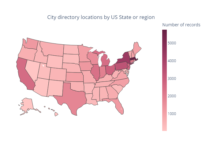
Visualize the data

Finally we will visualize the location data on a map.

from collections import Counter
from IPython.display import Image
import plotly.express as px         # For displaying charts and graphs

us_state_to_abbrev = {
    "Alabama": "AL", "Alaska": "AK", "Arizona": "AZ", "Arkansas": "AR", "California": "CA", "Colorado": "CO",
    "Connecticut": "CT", "Delaware": "DE", "Florida": "FL", "Georgia": "GA", "Hawaii": "HI", "Idaho": "ID",
    "Illinois": "IL", "Indiana": "IN", "Iowa": "IA", "Kansas": "KS", "Kentucky": "KY", "Louisiana": "LA",
    "Maine": "ME", "Maryland": "MD", "Massachusetts": "MA", "Michigan": "MI", "Minnesota": "MN", "Mississippi": "MS",
    "Missouri": "MO", "Montana": "MT", "Nebraska": "NE", "Nevada": "NV", "New Hampshire": "NH", "New Jersey": "NJ",
    "New Mexico": "NM", "New York": "NY", "North Carolina": "NC", "North Dakota": "ND", "Ohio": "OH", "Oklahoma": "OK",
    "Oregon": "OR", "Pennsylvania": "PA", "Rhode Island": "RI", "South Carolina": "SC", "South Dakota": "SD",
    "Tennessee": "TN", "Texas": "TX", "Utah": "UT", "Vermont": "VT", "Virginia": "VA", "Washington": "WA",
    "West Virginia": "WV", "Wisconsin": "WI", "Wyoming": "WY", "District of Columbia": "DC", "American Samoa": "AS",
    "Guam": "GU", "Northern Mariana Islands": "MP", "Puerto Rico": "PR", "United States Minor Outlying Islands": "UM",
    "U.S. Virgin Islands": "VI"
}

locations = df_by_location['State_region'] # Get a list of all the states/regions
locations_abbrev = [us_state_to_abbrev[loc] for loc in locations if loc in us_state_to_abbrev.keys()] # Convert to abbreviations
counter = Counter(locations_abbrev) # Count them
location_list = list(counter.keys())
counts = list(counter.values())

# Visualize it on a map
fig = px.choropleth(locations=location_list, locationmode="USA-states", color=counts, scope="usa",
                        color_continuous_scale=px.colors.sequential.Burg, labels={'color': 'Number of records'})
fig.update_layout(
        title=dict(text=f'City directory locations by US State or region', yanchor='top', xanchor='center', y=.9, x=.5),
        margin=dict(l=0, r=0, t=0, b=0, pad=0),
        coloraxis=dict(colorbar=dict(thickness=15, len=.75, xpad=5)),
        width=660
    )
Image(fig.to_image(format="png"))