LoC Data Package Tutorial: Digitized Telephone Directories Data Package

This notebook will demonstrate basic usage of using Python for interacting with data packages from the Library of Congress via the Digitized Telephone Directories Data Package which is derived from the Library’s U.S. Telephone Directory Collection. We will:

1. Output a summary of the contents of this data package

2. Read and query metadata from a data package

3. Download full text files and visualize it

Prerequisites

In order to run this notebook, please follow the instructions listed in this directory’s README.

Output data package summary

First we will output a summary of the Digitized Telephone Directories Data Package contents

import io

import pandas as pd                     # for reading, manipulating, and displaying data
import requests

from helpers import get_file_stats

DATA_URL = 'https://data.labs.loc.gov/telephone/' # Base URL of this data package

# Download the file manifest
file_manifest_url = f'{DATA_URL}manifest.json'
response = requests.get(file_manifest_url, timeout=60)
response_json = response.json()
files = [dict(zip(response_json["cols"], row)) for row in response_json["rows"]] # zip columns and rows

# Convert to Pandas DataFrame and show stats table
stats = get_file_stats(files)
pd.DataFrame(stats)

	FileType	Count	Size
0	.txt	486	2.37GB

Query the metadata in a data package

Next we will download a data package’s metadata, print a summary of the items’ subject values, then filter by a particular location.

All data packages have a metadata file in .json and .csv formats. Let’s load the data package’s metadata.json file:

metadata_url = f'{DATA_URL}metadata.json'
response = requests.get(metadata_url, timeout=60)
data = response.json()
print(f'Loaded metadata file with {len(data):,} entries.')

Loaded metadata file with 3,511 entries.

Next let’s convert to pandas DataFrame and print the available properties

df = pd.DataFrame(data)
print(', '.join(df.columns.to_list()))

Date_text, Date, Digitized, Id, IIIF_manifest, Preview_url, Call_number, Type_of_resource, Genre, Location_text, Original_format, Repository, Rights, Source_collection, Title, Mime_type, Online_format, Part_of, Number_of_files, Shelf_id, Url, Last_updated_in_api, Language, Location, Location_ocr

Next print the top 10 most frequent Locations in this dataset

# Since "Locations" are a list, we must "explode" it so there's just one location per row
# We convert to DataFrame so it displays as a table
df['Location_text'].explode().value_counts().iloc[:10].to_frame()

	Location_text
United States -- Illinois -- Chicago	131
United States -- Pennsylvania -- Philadelphia	113
United States -- California -- Los Angeles Central Area	97
United States -- Alabama -- Birmingham	74
United States -- California -- Oakland	74
United States -- California -- San Francisco	71
United States -- Maryland -- Baltimore	63
United States -- California -- Sacramento	51
United States -- California -- San Diego County	47
United States -- Georgia -- Atlanta	46

Now we filter the results to only those items with Location “United States – Alabama – Birmingham”

df_by_location = df.explode('Location_text')
subset = df_by_location[df_by_location.Location_text == 'United States -- Alabama -- Birmingham']
print(f'Found {subset.shape[0]:,} items with location "United States -- Alabama -- Birmingham"')

Found 74 items with location "United States -- Alabama -- Birmingham"

Download full text files and visualize it

First we merge the subset with the text files from the manifest

df_files = pd.DataFrame(files) # Convert file manifest to DataFrame
subset_with_text = pd.merge(df_files, subset, left_on='item_id', right_on='Id', how='inner')
print(f'Found {subset_with_text.shape[0]:,} Birmingham items with text files')

Found 74 Birmingham items with text files

Next we load the OCR text

text = ''
for i, row in subset_with_text.iterrows():
    file_url = f'https://{row["object_key"]}'
    response = requests.get(file_url, timeout=60)
    text += response.text
    text += '\n'
print(f"Loaded text string of length {len(text):,}")

Loaded text string of length 308,204,743

And clean up the text by removing non-words

import re

whitespace_pattern = re.compile(r"\s+")
nonword_pattern = re.compile(r" [\S]*[\\\^<>]+[\S]* ")
tinyword_pattern = re.compile(r" [\S][\S]?[\S]? ")
text = text.replace('\\n', '')
text = whitespace_pattern.sub(" ", text).strip()
text = nonword_pattern.sub(" ", text)
text = tinyword_pattern.sub(" ", text)
text = whitespace_pattern.sub(" ", text).strip()
print(text[:100])

LIBRARY CONGRESS PRESERVATION MICROFILMING PROGRAM MATERIAL WHICH FOLLOWS FROM COMBINED COLLECTIONS 

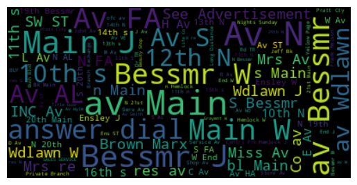
Finally generate a wordcloud using the text

import matplotlib.pyplot as plt         # for displaying data
from wordcloud import WordCloud

# Generate a word cloud image
wordcloud = WordCloud(max_font_size=40).generate(text)
plt.imshow(wordcloud, interpolation='bilinear')
plt.axis("off")

(-0.5, 399.5, 199.5, -0.5)