LoC Data Package Tutorial: National Jukebox collection

This notebook will demonstrate basic usage of using Python for interacting with data packages from the Library of Congress via the National Jukebox data package which is derived from the Library’s National Jukebox Collection. We will:

1. Output a summary of the contents of this data package

2. Read and query metadata from a data package

3. Download an audio file and visualize it

Prerequisites

In order to run this notebook, please follow the instructions listed in this directory’s README.

Output data package summary

First we will output a summary of the National Jukebox data package contents

import io

import pandas as pd                     # for reading, manipulating, and displaying data
import requests

from helpers import get_file_stats

DATA_URL = 'https://data.labs.loc.gov/jukebox/' # Base URL of this data package

# Download the file manifest
file_manifest_url = f'{DATA_URL}manifest.json'
response = requests.get(file_manifest_url, timeout=60)
response_json = response.json()
files = [dict(zip(response_json["cols"], row)) for row in response_json["rows"]] # zip columns and rows

# Convert to Pandas DataFrame and show stats table
stats = get_file_stats(files)
pd.DataFrame(stats)

	FileType	Count	Size
0	.mp3	5,882	17.0GB

Query the metadata in a data package

Next we will download a data package’s metadata, print a summary of the items’ subject values, then filter by a particular subject.

All data packages have a metadata file in .json and .csv formats. Let’s load the data package’s metadata.json file:

metadata_url = f'{DATA_URL}metadata.json'
response = requests.get(metadata_url, timeout=60)
data = response.json()
print(f'Loaded metadata file with {len(data):,} entries.')

Loaded metadata file with 5,882 entries.

Next let’s convert to pandas DataFrame and print the available properties

df = pd.DataFrame(data)
print(', '.join(df.columns.to_list()))

Date, Description, Digitized, Id, IIIF_manifest, Preview_url, Audio_type, Contributors, Genre, Language, Media_size, Recording_catalog_number, Date_text, Recording_label, Location_text, Recording_matrix_number, Recording_take_id, Recording_take_number, Rights, Mime_type, Online_format, Original_format, Part_of, Repository, Number_of_files, Shelf_id, Subjects, Last_updated_in_api, Title, Type_of_resource, Url, Source_collection, Location

Next print the top 10 most frequent Subjects in this dataset

# Since "Subjects" are a list, we must "explode" it so there's just one subject per row
# We convert to DataFrame so it displays as a table
df['Subjects'].explode().value_counts().iloc[:10].to_frame()

	Subjects
Victor	5882
Vocal	3763
Popular music	2479
Instrumental	1870
Opera	933
Classical music	719
Ethnic characterizations	482
Musical theater	430
Humorous songs	423
Ethnic music	299

Now we filter the results to only those items with subject “Opera”

df_by_subject = df.explode('Subjects')
opera_set = df_by_subject[df_by_subject.Subjects == 'Opera']
print(f'Found {opera_set.shape[0]:,} items with subject "Opera"')

Found 933 items with subject "Opera"

Download an audio file and visualize it

First we will merge the metadata with the file manifest to link the file URL to the respective item.

df_files = pd.DataFrame(files)
opera_set_with_audio = pd.merge(opera_set, df_files, left_on='Id', right_on='item_id', how='inner')
print(f'Found {opera_set_with_audio.shape[0]:,} opera items with audio files')

Found 933 opera items with audio files

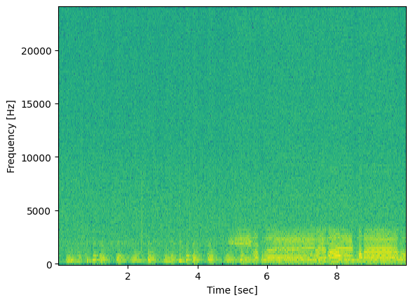
Finally we will download the first audio file, then display its spectrogram

import io

import matplotlib.pyplot as plt         # for displaying data
import numpy as np
from pydub import AudioSegment          # for reading and manipulating audio files
from scipy import signal                # for visualizing audio

item = opera_set_with_audio.iloc[0]
file_url = f'https://{item["object_key"]}'

# Downoad the audio to memory
response = requests.get(file_url, timeout=60)
audio_filestream = io.BytesIO(response.content)

# Read as mp3
sample_rate = 48000
sample_width = 1
channels = 1
sound = AudioSegment.from_mp3(audio_filestream)
sound = sound.set_channels(channels)
sound = sound.set_sample_width(sample_width)
sound = sound.set_frame_rate(sample_rate)

# Get the first 10 seconds
ten_seconds = 10 * 1000
first_10_seconds = sound[:ten_seconds]

# Get audio samples and sample rate
samples = first_10_seconds.get_array_of_samples()
samples = np.array(samples)

# Visualize the results
frequencies, times, spectrogram = signal.spectrogram(samples, sample_rate)
plt.pcolormesh(times, frequencies, np.log(spectrogram))
# plt.imshow(spectrogram)
plt.ylabel('Frequency [Hz]')
plt.xlabel('Time [sec]')
plt.show()